Menu Monday - Sort

Using the "Sort" functionality in Excel is an excellent way to help organize your data set.  It's very useful in sorting either alphabetical values or numeric values.  You can also get fancy and sort by things such as cell color, font color or cell icon :-)  The sort functions can be found on both the Home and Data tabs.

 Home Tab:

Data Tab:

 

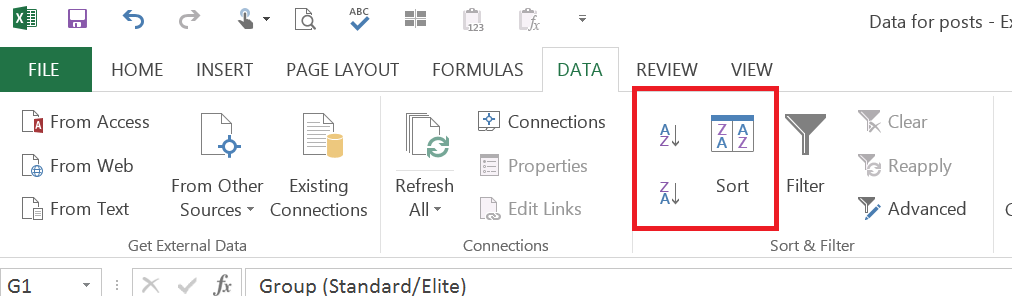
On each of these tabs, Excel gives 3 different options (icons) to use for sorting

1. Sort Lowest to Highest.  Excel will automatically sort the data using the column your cell is in as the column to sort by.  It will automatically determine the data set to be used.

 

2. Sort Highest to Lowest.  Excel will automatically sort the data using the column your cell is in as the column to sort by.  It will automatically determine the data set to be used.

 

3. Custom Sort. When you click on this icon, a window will pop up to let you customize what and how the data is to be sorted.  Using this option will let you sort by more than one column which can be very beneficial.

Example 1:

- In this scenario, I want to sort the data by the Contribution Amount and I want the values sorted lowest to highest.

- Click on any cell in column F, within the data set.  I chose to click on cell F3.

- Click on the Data tab

- Click on Sort Smallest to Largest (Lowest to Highest) icon.

- Excel automatically assumes that I want to sort the data in cells A1 through G10 and uses column F as the column to sort by from the smallest value on top to the highest value on the bottom.

- The data is now sorted based on column F

 

Example 2:

- In this scenario, I want to sort the data by Group and I want the values sorted highest to lowest as I want to see the Standard group first.

 

- Click on any cell in column G, within the data set.  I chose to click on cell G6.

- Click on the Data tab

- Click on Sort Z to A (Highest to Lowest) icon.

=

- Excel automatically assumes that I want to sort the data in cells A1 through G10 and uses column G as the column to sort by from the highest value on top to the lowest value on the bottom.

- The data is now sorted based on column G

 

Example 3:

- In this scenario, I want to sort the data by Name and I want the values sorted lowest to highest.  In order to do this I will need to sort on both the Last Name and First Name columns.

- Highlight cells A1 through G10

- Click on the Data tab

- Click on the Sort icon.

 

- A new window will pop up to allow customization of sorting

1. In the drop down under Column, choose Last Name

2. In the drop down under Sort On, choose Values

3. In the drop down under Order, choose A to Z

4. Click on Add Level to add another column to sort by

5. In the drop down under Column, choose First Name

6. In the drop down under Sort On, choose Values

7. In the drop down under Order, choose A to Z

8. Click OK

 

- The data is now sorted by Last Name and then by First Name

  



 Excel ya later!

Formula Friday - IF

One of the formulas I tend to use quite often in Excel is the "IF" formula.  The "IF" formula can be very helpful when trying to sort out your data.  The "IF" formula is very flexible as it lets you put in an argument to test and lets you determine what result is shown if the argument is true or false.  In this post I am going to give an example of a simple "IF" formula.  In the future I will give an example of using an "IF" formula, combined with other logical formula(s) to show what great things can be done with "IF"!

To use this formula:

-Click on the cell where you want to see the logical test results

-Enter =IF([logical test],[true value to display],[false value to display])

-Note: If you want to use a value as your true or false result, you will need to put "" around the value, i.e. "blue"

-Press Enter

-Now you will see the result

Example:

-In this example I have a list of individuals who have donated money to a charity.  I want to break the list down into 2 groups based on the dollar amount given.  Those individuals who gave more $100 will be in the Elite group.  The individuals who gave $100 or less will be in the Standard group.

 

-Click on Cell G2

-In cell G2, enter =IF(F2>100,"Elite","Standard")

 

1. In this case I am looking at the value in column F to determine which group the individual belongs in, so I use column F in my logical test.  I am using F2>100, because anything where the value in column F is greater than 100, I want column G to show Elite.

2. If my statement is true (the value in F is greater than 100), then the cell in column G will return "Elite"

3. If my statement is false (the value in F is less than or equal to 100), then the cell in column G will return "Standard"

-Press Enter

-Now I see the result of "Elite" in cell G2 since the Contribution amount in cell F2 was greater than 100

 

-To finish this example, I want to copy the formula to the remainder of the contributors to figure out the groupings.  Therefore, I need to copy this formula down to cells G3 through G10.

-Copy cell G2

-Highlight cells G3 through G10

-Paste the formula

-Now each of these cells will have the same formula and will display the result in each cell

-Cells with formulas

 

-Results

 

Excel ya later!

Formula Friday - LEN (cell character length)

Do you need to know how many characters are in a certain cell in Excel?  Well, Excel has an easy formula you can use to count the characters or see the length.  The formula is LEN.  An example of when this can come in really handy is when you are filling in a form or uploading data to a form that has specific character limits.

To use this formula:

-Click on the cell where you want to see the character count (length) results

-Enter LEN([cell you want evaluated])

-Note: Spaces will also be counted as a character with this formula

-Press Enter

-Now you will see the number of characters in the result cell

Example:

-In this example I want to see how many characters are in each of the cells in the Address column.  The form that I am uploaded my data to has a character limit of 20 for the address field, so I want to make sure that my cells do not exceed this count.

 

-Click on cell G2

 

-Enter =LEN(C2)

-Press Enter

-Now you will see the number of characters in cell G2 (12 characters)

-From here I am going to copy this formula down to cells G3 through G10.

-Copy cell G2

-Highlight cells G3 through G10

-Paste the formula

-Now each of these cells will have the same formula and will display the characters in each cell

-Cells G6 and G10 have more than 20 characters, so now I know I need to make some changes to those cells

Excel ya later!

 

Menu Monday - Conditional Formatting - Duplicates (Highlight Duplicates)

In an earlier post, I went through the steps of using the Remove Duplicates function in Excel.  This is great if you want to completely remove the duplicate values.  But what if you want to just find the duplicate values in your data set?  There are some formulas you could use to do this, but another easy way to do it is to use the Conditional Formatting function.

To use this function:

-Highlight the cells where you want to find the duplicate values

-The cells can be in multiple rows/columns and do not have to be adjacent to one another

-Click on the Home tab

-In the Styles section, click on the Conditional Formatting drop-down menu

-Hover over "Highlight Cell Rules"

-Click on "Duplicate Values…"

-A new window will pop up to ask how you would like the cells formatted

-Leave the left drop-down menu on "Duplicate"

-The right drop-down menu can be left alone if you are ok with the default formatting, or you can click on the drop-down menu to adjust the formatting

-There are multiple default formats, otherwise you can click on "Custom Format" to create your own

-Once you have made your formatting choice, click OK

-Now, looking at your data set, you should see the duplicate values formatted in the way you chose

Example 1:

-In this scenario, I want to highlight where I have duplicate names in my data set

-Highlight cells A2 through A1

-Click on the Home tab

-In the Styles section, click on the Conditional Formatting drop-down menu [1]

-Hover over "Highlight Cell Rules" [2]

-Click on "Duplicate Values…" [3]

 

-A new window will pop up to ask how you would like the cells formatted

-Leave the left drop-down menu on "Duplicate" [1]

-In this scenario, I am ok with the default formatting on the right drop-down to have the cells filled with light red and have dark red text [2]

-Click OK [3]

-Now the duplicate names are highlighted in red and have red text

 

Example 2:

-In this scenario, I want to highlight where I have duplicates in List 1 and List 2

-Highlight cells A2 through B8

-Click on the Home tab

-In the Styles section, click on the Conditional Formatting drop-down menu [1]

-Hover over "Highlight Cell Rules" [2]

-Click on "Duplicate Values…" [3]

-A new window will pop up to ask how you would like the cells formatted

-Leave the left drop-down menu on "Duplicate" [1]

-In this scenario, I am ok with the default formatting on the right drop-down to have the cells filled with light red and have dark red text [2]

-Click OK [3]

-Now the duplicate shapes are highlighted in red and have red text

 

Excel ya later!

Formula Friday - COUNTA (Count non-blank cells)

An easy way to count cells that have data in Excel is by using the 'COUNTA' formula.  This formula will count cells that are not blank, whether they are numeric or anything else.  This is different from the COUNT formula that only counts cells if they have a number in them.

To use this formula:

-Click on the cell where you want to see the count results

-Enter COUNTA(Number1:Number2)

-The range of cells to be evaluated can be either consecutive or non-consecutive

-Like in other formulas, to evaluate consecutive cells, the cell range will use a ':' between cells

-i.e. COUNTA(B1:B15)

-To evaluate non-consecutive cells, the cells will be separated by a ','

-i.e. COUNTA(B1,B5,B8)

-Or, a combination can also be used

-i.e. COUNTA(B1:B5,B9)

-Press Enter

-Now you will see the number of non-blank cells in the result cell

Example:

-In this scenario, I want to count the number of months where the fruit or vegetable was tracked (has an "X" in the cell).

-I want the results to be displayed in row 17

-For this example, I will just focus on counting the Bananas to start with

-In cell B17, enter =COUNTA(B5:B16)

-Press Enter

-You will now see the result of 4 as there are 4 months that have an 'X" in the cell (January, June, August & November)

-Now I can copy this formula across to cells C17 through M17 to get the results for the other Fruits/Vegetables

-Results

 

Excel ya later!

Menu Monday - Merge & Center (Merge Cells)

When putting together a dashboard or a report, a function that can be very useful is the "Merge & Center" function.   Merge & Center will combine two or more adjacent cells to create one larger cell.  A great example of using this function is when you have a header that spans across multiple columns.

This function is useful when you want to merge the adjacent cells as well as center the text in them

-To use this function:

-Select the adjacent cells that you want merged together

-Note: The cells can be any combination of adjacent cells in the same row, adjacent cells in the same column, or adjacent cells in rows and columns

-Click on the Home tab

-Click on the Merge & Center icon in the Alignment section

-Click on Merge & Center

-Now you will see your text merged into one larger cell and centered

-Example 1

-In this scenario, I want to create a header in row 3 called "Fruit" that spans across columns B-G

-Select cells B3-G3

-Click on the Home tab

-Click on the Merge & Center icon in the Alignment section

-Click on Merge & Center

-Now you will see "Fruit" centered across cells B3-G3

-When you click in the cell it will now be one large cell

 

Excel ya later!

 

Formula Friday - Today and Now (Auto Populate the Date!)

Excel has built in two easy formulas that will automatically display the current date or current date and time in your spreadsheet.  Each of these formulas will recalculate each time your spreadsheet is either reopened or refreshed. 

1. TODAY

-This first option is to use the TODAY formula.  This formula will display the current date.

-To use this formula, enter 'TODAY()' in the cell where you want the date displayed

-Press Enter

-You will now see the date

-Example 1:

-In this example, I want to have the date auto populate in cell A2 each time the report is opened

-In cell A2 enter 'TODAY()'

-Press Enter

-The date will now appear in cell A2

 

2. NOW

-The second option is to use the NOW formula.  This formula will display the current date and time.

-To use this formula, enter 'NOW()' in the cell where you want the date and time displayed

-Press Enter

-You will now see the date and time

-Example 2:

-In this example, I want to have the date and time auto populate in cell A2 each time the report is opened

-In cell A2 enter 'NOW()' and press Enter

-The date and time will now appear in cell A2

 

Reminder: Each of these formulas will recalculate each time the spreadsheet is reopened or the sheet is recalculated.

Excel ya later!