Menu Monday - Sort

Using the "Sort" functionality in Excel is an excellent way to help organize your data set.  It's very useful in sorting either alphabetical values or numeric values.  You can also get fancy and sort by things such as cell color, font color or cell icon :-)  The sort functions can be found on both the Home and Data tabs.

 Home Tab:

Data Tab:

 

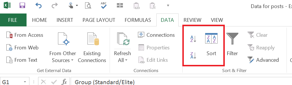
On each of these tabs, Excel gives 3 different options (icons) to use for sorting

1. Sort Lowest to Highest.  Excel will automatically sort the data using the column your cell is in as the column to sort by.  It will automatically determine the data set to be used.

 

2. Sort Highest to Lowest.  Excel will automatically sort the data using the column your cell is in as the column to sort by.  It will automatically determine the data set to be used.

 

3. Custom Sort. When you click on this icon, a window will pop up to let you customize what and how the data is to be sorted.  Using this option will let you sort by more than one column which can be very beneficial.

Example 1:

- In this scenario, I want to sort the data by the Contribution Amount and I want the values sorted lowest to highest.

- Click on any cell in column F, within the data set.  I chose to click on cell F3.

- Click on the Data tab

- Click on Sort Smallest to Largest (Lowest to Highest) icon.

- Excel automatically assumes that I want to sort the data in cells A1 through G10 and uses column F as the column to sort by from the smallest value on top to the highest value on the bottom.

- The data is now sorted based on column F

 

Example 2:

- In this scenario, I want to sort the data by Group and I want the values sorted highest to lowest as I want to see the Standard group first.

 

- Click on any cell in column G, within the data set.  I chose to click on cell G6.

- Click on the Data tab

- Click on Sort Z to A (Highest to Lowest) icon.

=

- Excel automatically assumes that I want to sort the data in cells A1 through G10 and uses column G as the column to sort by from the highest value on top to the lowest value on the bottom.

- The data is now sorted based on column G

 

Example 3:

- In this scenario, I want to sort the data by Name and I want the values sorted lowest to highest.  In order to do this I will need to sort on both the Last Name and First Name columns.

- Highlight cells A1 through G10

- Click on the Data tab

- Click on the Sort icon.

 

- A new window will pop up to allow customization of sorting

1. In the drop down under Column, choose Last Name

2. In the drop down under Sort On, choose Values

3. In the drop down under Order, choose A to Z

4. Click on Add Level to add another column to sort by

5. In the drop down under Column, choose First Name

6. In the drop down under Sort On, choose Values

7. In the drop down under Order, choose A to Z

8. Click OK

 

- The data is now sorted by Last Name and then by First Name

  



 Excel ya later!

Menu Monday - Conditional Formatting - Duplicates (Highlight Duplicates)

In an earlier post, I went through the steps of using the Remove Duplicates function in Excel.  This is great if you want to completely remove the duplicate values.  But what if you want to just find the duplicate values in your data set?  There are some formulas you could use to do this, but another easy way to do it is to use the Conditional Formatting function.

To use this function:

-Highlight the cells where you want to find the duplicate values

-The cells can be in multiple rows/columns and do not have to be adjacent to one another

-Click on the Home tab

-In the Styles section, click on the Conditional Formatting drop-down menu

-Hover over "Highlight Cell Rules"

-Click on "Duplicate Values…"

-A new window will pop up to ask how you would like the cells formatted

-Leave the left drop-down menu on "Duplicate"

-The right drop-down menu can be left alone if you are ok with the default formatting, or you can click on the drop-down menu to adjust the formatting

-There are multiple default formats, otherwise you can click on "Custom Format" to create your own

-Once you have made your formatting choice, click OK

-Now, looking at your data set, you should see the duplicate values formatted in the way you chose

Example 1:

-In this scenario, I want to highlight where I have duplicate names in my data set

-Highlight cells A2 through A1

-Click on the Home tab

-In the Styles section, click on the Conditional Formatting drop-down menu [1]

-Hover over "Highlight Cell Rules" [2]

-Click on "Duplicate Values…" [3]

 

-A new window will pop up to ask how you would like the cells formatted

-Leave the left drop-down menu on "Duplicate" [1]

-In this scenario, I am ok with the default formatting on the right drop-down to have the cells filled with light red and have dark red text [2]

-Click OK [3]

-Now the duplicate names are highlighted in red and have red text

 

Example 2:

-In this scenario, I want to highlight where I have duplicates in List 1 and List 2

-Highlight cells A2 through B8

-Click on the Home tab

-In the Styles section, click on the Conditional Formatting drop-down menu [1]

-Hover over "Highlight Cell Rules" [2]

-Click on "Duplicate Values…" [3]

-A new window will pop up to ask how you would like the cells formatted

-Leave the left drop-down menu on "Duplicate" [1]

-In this scenario, I am ok with the default formatting on the right drop-down to have the cells filled with light red and have dark red text [2]

-Click OK [3]

-Now the duplicate shapes are highlighted in red and have red text

 

Excel ya later!

Menu Monday - Merge & Center (Merge Cells)

When putting together a dashboard or a report, a function that can be very useful is the "Merge & Center" function.   Merge & Center will combine two or more adjacent cells to create one larger cell.  A great example of using this function is when you have a header that spans across multiple columns.

This function is useful when you want to merge the adjacent cells as well as center the text in them

-To use this function:

-Select the adjacent cells that you want merged together

-Note: The cells can be any combination of adjacent cells in the same row, adjacent cells in the same column, or adjacent cells in rows and columns

-Click on the Home tab

-Click on the Merge & Center icon in the Alignment section

-Click on Merge & Center

-Now you will see your text merged into one larger cell and centered

-Example 1

-In this scenario, I want to create a header in row 3 called "Fruit" that spans across columns B-G

-Select cells B3-G3

-Click on the Home tab

-Click on the Merge & Center icon in the Alignment section

-Click on Merge & Center

-Now you will see "Fruit" centered across cells B3-G3

-When you click in the cell it will now be one large cell

 

Excel ya later!

 

Menu Monday - Freeze Panes

When you are working with large data sets in Excel, a wonderful function to consider using is the 'Freeze Panes' function.  This function is especially useful when you have row and/or column headings that you want to continue to see as you scroll through your data.  Excel gives 3 options for 'Freeze Panes':

1. Freeze Panes

-This function is useful when you want to freeze both rows and columns and/or have multiple rows and/or columns to freeze.  Basically this function allows you to choose which data you want to freeze versus the other two options below where Excel automatically freezes certain rows/columns.

-To use this function:

- Click on the cell where you want the following to happen:

1. The row(s) above the selected cell will be frozen (the cells must be visible on the page at this time)

2. The column(s) to the left of the selected cell will be frozen

-Click on the View Tab

-Click on 'Freeze Panes' in the Window section

-You will be given 3 choices, click 'Freeze Panes' from the menu

-Now when you scroll, any cells that were above or to the left of your selected cell should not move

-Example 1

-In this scenario, I want to freeze the first 2 rows and the first column as they are headers

-Click on cell B3

-Click on the View tab

-In the Window section click on 'Freeze Panes' icon

-Click on 'Freeze Panes' from the Freeze Panes menu

-Now when you scroll down, you will still see your top to rows

-Next, scroll to the right and you will still see your first column on the left

 

2. Freeze Top Row

-This function is useful when you just want to freeze the first row of your data

-To use this function:

-Click in any cell on your spreadsheet (no specific cell is needed)

-Click on the View Tab

-Click on 'Freeze Panes' in the Window section

-You will be given 3 choices, click 'Freeze Top Row' from the menu

-Now when you scroll, the first row will not move

-Example 2

-In this scenario, I want to freeze only the top row so that I can see the header as I scroll down through the weeks

-Click on any cell in the spreadsheet

-Click on the View tab

-In the Window section click on 'Freeze Panes' icon

-Click on 'Freeze Top Row' from the Freeze Panes menu

-Now when you scroll down, you will continue to see your top row

 

3. Freeze First Column

-This function is useful when you just want to freeze the first column of your data

-To use this function:

-Click in any cell on your spreadsheet (no specific cell is needed)

-Click on the View Tab

-Click on 'Freeze Panes' in the Window section

-You will be given 3 choices, click 'Freeze First Column' from the menu

-Now when you scroll, the first column will not move

-Example 3

-In this scenario, I want to freeze only the first column so that I can see the header as I scroll to the right

-Click on any cell in the spreadsheet

-Click on the View tab

-In the Window section click on 'Freeze Panes' icon

-Click on 'Freeze First Column' from the Freeze Panes menu

-Now when you scroll to the right, you will continue to see your first column

 

Now, we've walked through the steps on how to freeze panes, but what if you want to unfreeze the panes?  In any of the above 3 scenarios, if you want to unfreeze the panes, follow the steps below:

-Click in any cell on your spreadsheet (no specific cell is needed)

-Click on the View Tab

-Click on 'Freeze Panes' in the Window section

-You will be given 3 choices, click 'Unfreeze Panes' from the menu

Excel ya later!

Formula Friday - Random Number Generator

Do you need to quickly produce a random number?  Excel has two simple formulas that will quickly generate a random number. 

1. RAND
• The first option is to use the RAND formula.  This formula will generate a number greater than or equal to 0 and less than 1. 
• To use this formula, enter '=RAND()' in the cell where you want the random number

• Press Enter
• You will now see a random number

 

• Note: Each time the spreadsheet is recalculated, the number will change

2. RANDBETWEEN
• The second option is to use the RANDBETWEEN formula.  With this formula, a random number will be generated between 2 numbers that you identify.
• Note: The result from this formula will be an integer
• To use this formula, enter 'RANDBETWEEN(Number1,Number2)
• Number1 is the lowest number
• Number2 is the highest number
• Press Enter
• You will now see a random number
• Note: Each time the spreadsheet is recalculated, the number will change
• Example 1
• I am looking for a number between 1 and 20
• In cell A1, enter RANDBETWEEN(1,20)

• Press Enter
• An integer between 1 and 20 is generated

 

 

Once you have the formula in place, if you want to regenerate the random number, you can press F9 or click "Calculate Now" on the Formula tab in the Calculation section.

 

 

As I explained with the Sum formula, there are multiple ways to insert the formulas into the spreadsheet.

1. Type the formula in as described above
2. Use the "Insert Icon" function and type in either RAND or RANDBETWEEN

 

3. On the Formulas tab, click on the Math & Trig drop down in the Function Library section and scroll down to find either RAND or RANDBETWEEN

 

Example 2

• In this example I want a dollar amount between 1 and 10.  In this example, I am going to use a combination of the two formulas above as I want a number with decimals.  If I only wanted an integer, then I would just use the RANDBETWEEN formula.
• Insert  =RANDBETWEEN(1,10)+RAND() in the cell

• Press Enter
• Now Excel will generate a number between 1 and 10 and a number between 0 and 1 and add them together

 

Excel ya later!