Monday, March 10, 2014

Menu Monday - Remove Duplicates

Removing duplicates from a large list of data can be a daunting task, but now with the 'Remove Duplicates' function, it can be breeze.

To use the function, follow the steps below:

  • Highlight the cells where you want the duplicates removed
  • Click on the Data tab on the Ribbon (Menu)
  • Click on 'Remove Duplicates' in the Data Tools section
  • A Remove Duplicates window will pop-up
  • Make any adjustments as needed (see examples below)
  • Click OK
  • A window will pop-up to tell you how many duplicate values were removed and how many unique values remain
  • Click OK
  • Now you will see your list with only unique values
 
Example 1 - Single List

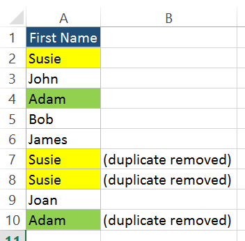
  • In this scenario, I have a single list of data containing first names.  I want only the unique values and want to remove any duplicates.


  • First, highlight cells A1:A10 (I could also just highlight all of column A by clicking on A if this is the only data in this column)


  • Click on the Data tab on the Ribbon (Menu)
  • Click on 'Remove Duplicates in the Data Tools section
  • A Remove Duplicates window will pop-up

  • In this case I only have 1 column of data, so I will leave the "First Name" column checked
  • I also had included the data header in the cells that I highlighted, so I will leave the "My data has headers" box checked
    • Note: If you do not have a header or did not include the header in your data, you will want to uncheck this box
  • Click OK
  • A window pops-up say that 3 duplicate values were found and removed and 6 unique values remain


  • Click OK
  • Now the list only contains 6 names instead of 9

  • Below is a visual of the data an what was removed
 

Example 2 - Multiple Columns of Data, Compare all columns
  • In this scenario, I have multiple columns of data containing names and addresses.  I want to remove the duplicates where the values in every column are duplicated.
 
  • First, highlight cells A1:E10 (I could also just highlight all of columns A-E if this is the only data in this column)
    • Note: Highlight all of the adjacent data so that it removes the entire row, even if you are not checking each column for duplicates

  • Click on the Data tab on the Ribbon (Menu)
  • Click on 'Remove Duplicates' in the Data Tools section
  • A Remove Duplicates window will pop-up
  • In this case I only want to remove the row if the data in each column is a duplicate, therefore I want to check all the boxes for each column (i.e. There are 3 Susie Smiths, but I only want to delete the data if the First Name, Last Name, Address, City and State are exactly the same.  So, in this scenario, only 1 of the Susie Smiths will be deleted as there are 2 with the same address and 1 with a different address.)
    • Note: See Example 3 if you don't want to compare all columns
  • I also had included the data header in the cells that I highlighted, so I will leave the "My data has headers" box checked
    • Note: If you do not have a header or did not include the header in your data, you will want to uncheck this box
  • Click OK
  • A window pops-up say that 2 duplicate values were found and removed and 7 unique values remain
 
  • Click OK
  • Now the list only contains 7 names instead of 9
    • Below is a visual of the data an what was removed


Example 3 - Multiple Columns of Data, Compare only First Name and Last Name

  • In this scenario, I have multiple columns of data containing names and addresses.  I want to remove the duplicates where the values in the First Name and Last Name columns are duplicated.
  • First, highlight cells A1:E10 (I could also just highlight all of columns A-E if this is the only data in this column)
    • Note: Highlight all of the adjacent data so that it removes the entire row, even if you are not checking each column for duplicates
  • Click on the Data tab on the Ribbon (Menu)
  • Click on 'Remove Duplicates' in the Data Tools section
 
  • A Remove Duplicates window will pop-up
  • In this scenario, I only want the boxes checked for First Name and Last Name as I am only comparing to see if there are duplicates in these columns (i.e. There are 3 Susie Smiths, so I want Excel to remove 2 of them even though 1 of the addresses is different)
  • I also had included the data header in the cells that I highlighted, so I will leave the "My data has headers" box checked
    • Note: If you do not have a header or did not include the header in your data, you will want to uncheck this box
  • Click OK
  • A window pops-up say that 3 duplicate values were found and removed and 6 unique values remain
  • Click OK
  • Now the list only contains 6 names instead of 9
 
  • Below is a visual of the data an what was removed
 
Excel ya later!

Friday, March 7, 2014

Formula Friday - Sum

Using the sum function in Excel is a convenient and quick way to add small or large data sets.  The function can be used to sum consecutive numbers or non-consecutive numbers.  There are at least 4 ways to insert the formula into your spreadsheet:

1. Type the formula into the cell that you want to show the summed result in:
    • For consecutive numbers
      • =sum(Number1:Number2)
      • Example 1:
        • In this example I want to sum the total units of Sunday through Saturday in cell B9
        • In order to do this, in cell B9 type '=SUM(B2:B8)' and press Enter
        • Once I hit Enter I get the result of 38
        • To see the formula, click back into cell B9 and you will see the formula in the Formula Bar
    • For non-consecutive numbers
      • =sum(Number1,Number2)
      • Example 2
        • In this example I want to sum only the units for Sunday and Saturday in cell B9
        • In order to do this, in cell B9 type '=SUM(B2,B8)' and press Enter
        • Once I hit Enter I get the result of 10
        • To see the formula, click back into cell B9 and you will see the formula in the Formula Bar
    •  For a combination of consecutive and non-consecutive numbers
      • Example 3
        • In this example I want to sum only the units for Friday, Saturday and Sunday in cell B9
        • In order to do this, in cell B9 type '=SUM(B2,B7:B8)' and press Enter
        • NOTE: The difference between the consecutive and non-consecutive numbers is the difference of using either ' : ' or ' , '.  For consecutive numbers, use the ' : ' between the first and last number. For non-consecutive numbers, use a ' , ' between the numbers.
        • Once I hit Enter I get the result of 13
        • To see the formula, click back into cell B9 and you will see the formula in the Formula Bar
        •  

2. The second option is to click on the "Insert Function" icon next to the Formula Bar
    • Once the icon is clicked, the Insert Function window will pop-up
      1. Type in the word "sum" in the "Search for a function:" box
      2. Click the "Go" button
      3. Select "Sum" in the "Select a function:" section
      4. Click the "OK" button
    •  Next, the Function Arguments window will pop up
    • There are 2 options of how to enter the cell data into this window
      1. Type in the cell data
        • Below is an screenshot of what Example 3 from above would look like

      2. Use the cell selector icon to choose the cells you want to sum
        • Click the icon
        • The window will minimize
        • Click on the cell or consecutive cells you want to sum
        • Click on the icon on the right once you have finished
        • Repeat these steps for any additional non-consecutive cell(s) in Number2, Number3, etc.
    • Click OK
The 3rd and 4th options work best for summing consecutive cells. That being said, you can make adjustments to the formula to sum non-consecutive cells or a combination of both.
 
3. The 3rd option is to use the AutoSum function on the Home tab
  • Click on the cell that you want to display the summed result (which is usually best if it is adjacent to the data you want summed)
  • Click on the Home tab
  • Click on the AutoSum function in the Editing section
  • Excel will automatically add in the Sum formula and sum the adjacent cells
  • In this example, I want the summed total in cell C9
  • While in C9, I clicked on the AutoSum function on the Home Menu
  • Excel automatically entered the sum formula in C9 and assumed I wanted to sum the adjacent cells
  • If I am ok with the formula, I click Enter
  • If I want to make changes to the formula, I click into the cell to make changes, then press Enter
4. Finally, the 4th option I have is to use the AutoSum function on the Formulas tab in the Function Library
  •  Follow the same steps as you would in Option 3
 
Excel ya later!
 

Tuesday, March 4, 2014

Menu Monday - Format Painter

Do you like the format settings you have set up for a certain cell and want those same exact settings for another cell(s)?  Well, if so, the Format Painter function is your new best friend. 

There are 2 options when using the Format Painter function:
  1. Copy the format settings to one cell or one selection of cells.  
  2.  
    • In order to do this, click on the cell that has the format settings you are seeking
    • Click on the Home tab on the Ribbon (Menu)
    • In the Clipboard section on the very left, click on the Format Painter icon
    • Next, click on the cell or selection of cell(s) that you want to be formatted
    • You should now see the cells adjusted to the new format
    • Example 1:
      • In this scenario I want to change Wednesday to be the same formatting as Sunday
      • First, select cell A1 for Sunday
      • Next, click on the Home tab on the Ribbon and click on the Format Painter icon
      •  
      • Now click on cell A4 to change the formatting of Wednesday
    • Example 2:
      • In this scenario I want to change Wednesday through Friday to be the same formatting as Sunday
      • First, select cell A1 for Sunday
      • Next, click on the Home tab on the Ribbon and click on the Format Painter icon
      •  
      • Now highlight cells A4 through A6 to change the formatting of Wednesday through Friday
  3. Copy the format settings to multiple [disconnected] cells
    • In order to do this, click on the cell that has the format settings you are seeking
    • Click on the Home tab on the Ribbon (Menu)
    • In the Clipboard section on the very left, double-click on the Format Painter icon
    • Next, click on the cells that you want to be formatted
    • You should now see the cells adjusted to the new format
    • Either click the Esc key on the keyboard or click the Format Painter icon again when you are done formatting the cells
    • Example 3:
      • In this scenario I want to change Tuesday, Thursday and Saturday to be the same formatting as Sunday
      • First, select cell A1 for Sunday
      • Next, click on the Home tab on the Ribbon and double-click on the Format Painter icon
      •  
      • Now click on cells A3, A5, and A7 to change the formatting of Tuesday, Thursday and Saturday
      • Either click the Esc on the keyboard or click the Format Painter icon again when you are done formatting the cells
Excel ya later!